The only question that requires R this week is 1.3. Consequently, this homework does not have to be in the form of an R notebook. You should hand in a .pdf (either from Word, or a scan of handwritten answers).

Q1

Recall the parallel lines model from the meadowfoam case study \[ \mu\{\text{Flowers} \, | \, \text{light},\text{ early}\} = \beta_0 + \beta_1 \textit{light} + \beta_2 \textit{early} \] where early was an indicator variable that took on the value 0 if the unit started light treatment at PFI and 1 if the unit started light treatment 24 days prior to PFI.

An alternative approach would be to use the “days before PFI” as a continuous time variable. I.e. time = 24 for the units receiving light starting 24 days before PFI and time = 0 for the units receiving light treatment starting at PFI.

A model might then be

(I’ve used γs instead of βs here to indicate the parameters in this model may not take the same values as in the previous model.)

1. Calculate the effect of the time variable in the above multiple linear regression, in terms of the parameters.

2. An increase in time from 0 to 24 days is equivalent to an increase in early from 0 to 1, i.e. the change in mean number of flowers going from time = 0 to time = 24, should be the same as the change in mean number of flowers going from early = 0 to early = 1. Use this fact along with your answer to 1 to relate \(\beta_2\) to \(\gamma_2\).

3. Fit both models in R, and use the estimated parameters to confirm your finding in 2. You’ll need to create the time variable:

load(url("http://stat512.cwick.co.nz/data/case0901.rda"))
case0901$time <- ifelse(case0901$Time == "Early", 24, 0)

Q2

Another alternative to the parallel straight lines model would be to use a set of indicator variables for light intensity \[ \mu\{\text{Flowers} | \text{light},\text{ early}\} = \beta_0 + \beta_1 \textit{L300} + \beta_2 \textit{L450}+ \beta_3 \textit{L600}+ \beta_4 \textit{L750}+ \beta_5 \textit{L900}+ \beta_6 \textit{early} \] where L300 is an indicator variable for the Intensity being 300 μmol/m2/sec, L450 is an indicator variable for the Intensity being 450 μmol/m2/sec and so on.

1. Using the above model, find the mean number of flowers for the following treatment combinations, in terms of the parameters.
   • 150 μmol/m2/sec, 24 days before PFI (i.e. early = 1).
   • 150 μmol/m2/sec, at PFI (i.e. early = 0).
   • 450 μmol/m2/sec, 24 days before PFI (i.e. early = 1).
   • 450 μmol/m2/sec, at PFI (i.e. early = 0).

2. Timing could be allowed to interact with the indicator variables for Intensity using the following model \[ \mu\{\text{Flowers} | \text{Intensity},\text{ early}\} = \beta_0 + \beta_1 \textit{L300} + \beta_2 \textit{L450}+ \beta_3 \textit{L600}+ \beta_4 \textit{L750}+ \beta_5 \textit{L900}+ \beta_6 \textit{early} + \\ \beta_7 \textit{L300}\times\textit{early} + \beta_8 \textit{L450}\times\textit{early}+ \beta_9 \textit{L600}\times\textit{early}+ \beta_{10} \textit{L750}\times\textit{early}+ \beta_{11}\textit{L900}\times\textit{early} \] Using the this model, find the mean number of flowers for the following treatment combinations. * 150 μmol/m2/sec, 24 days before PFI (i.e. early = 1). * 150 μmol/m2/sec, at PFI (i.e. early = 0). * 450 μmol/m2/sec, 24 days before PFI (i.e. early = 1). * 450 μmol/m2/sec, at PFI (i.e. early = 0).

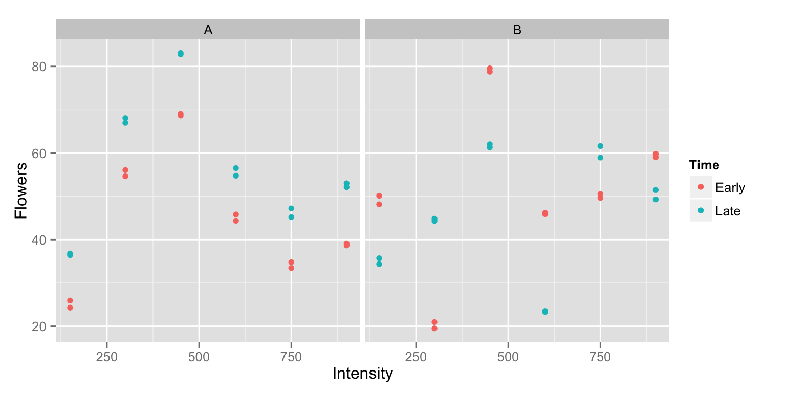
3. The following two plots represent ideal realizations under the above two models. Which plot corresponds to which model? (It might help to calculate the effect of early in the two models.)

Q3

9.19 in Sleuth

Has homework got you down? It could be worse. Depression, like other illnesses is more prevalent among adults with less education than you have.

R. A. Miech and M. J. Shanahan investigated the association of depression with age and education, based on a 1990 nationwide telephone survey of 2,031 adults aged 18 to 90. Of particular interest was their finding that the association of depression with education strengthens with increasing age - a phenomenon they called “divergence hypothesis”.

They constructed a depression score from responses to several related questions. Education was categorized as (i) college degree, (ii) high school degree plus some college, or (iii) high school degree only.

1. Write down a linear regression model in which the mean depression score changes linearly with age in all three categories, with possibly unequal slopes and intercepts. Identify a single parameter that measures the diverging gap between categories (iii) and (i) with age. If you use indicator variables, make sure you define them.

2. Modify the model to specify that the slopes of the regression lines with age are equal in categories (i) and (ii) but possibly different in category (iii). Again identify a single parameter measuring divergence.